该系列为南京大学课程《用Python玩转数据》学习笔记,主要以思维导图的记录
8.1 线性回归分析入门之波士顿房价预测
获取数据
加载数据
1
2
3
4
5
6
from sklearn import datasets
import pandas as pd
boston = datasets.load_boston()
x = pd.DataFrame(boston.data, columns=boston.feature_names)
y = pd.DataFrame(boston.target, columns=['MEDV'])查看数据含义
1
2
3
4
5
6
7
8
9
10
11
12
13
14
15
16
17
18
19
20
21
22
23
24
25
26
27
28
29
30
31
32
33
34
35
36
37
38
print(boston.DESCR)
.. _boston_dataset:
Boston house prices dataset
---------------------------
**Data Set Characteristics:**
:Number of Instances: 506
:Number of Attributes: 13 numeric/categorical predictive. Median Value (attribute 14) is usually the target.
:Attribute Information (in order):
- CRIM per capita crime rate by town
- ZN proportion of residential land zoned for lots over 25,000 sq.ft.
- INDUS proportion of non-retail business acres per town
- CHAS Charles River dummy variable (= 1 if tract bounds river; 0 otherwise)
- NOX nitric oxides concentration (parts per 10 million)
- RM average number of rooms per dwelling
- AGE proportion of owner-occupied units built prior to 1940
- DIS weighted distances to five Boston employment centres
- RAD index of accessibility to radial highways
- TAX full-value property-tax rate per $10,000
- PTRATIO pupil-teacher ratio by town
- B 1000(Bk - 0.63)^2 where Bk is the proportion of blacks by town
- LSTAT % lower status of the population
- MEDV Median value of owner-occupied homes in $1000's
:Missing Attribute Values: None
:Creator: Harrison, D. and Rubinfeld, D.L.
This is a copy of UCI ML housing dataset.
https://archive.ics.uci.edu/ml/machine-learning-databases/housing/
This dataset was taken from the StatLib library which is maintained at Carnegie Mellon University.
The Boston house-price data of Harrison, D. and Rubinfeld, D.L. 'Hedonic
prices and the demand for clean air', J. Environ. Economics & Management,
vol.5, 81-102, 1978. Used in Belsley, Kuh & Welsch, 'Regression diagnostics
', Wiley, 1980. N.B. Various transformations are used in the table on
pages 244-261 of the latter.
The Boston house-price data has been used in many machine learning papers that address regression
problems.
.. topic:: References
- Belsley, Kuh & Welsch, 'Regression diagnostics: Identifying Influential Data and Sources of Collinearity', Wiley, 1980. 244-261.
- Quinlan,R. (1993). Combining Instance-Based and Model-Based Learning. In Proceedings on the Tenth International Conference of Machine Learning, 236-243, University of Massachusetts, Amherst. Morgan Kaufmann.
预判
绘制房间数[‘RM’]与房价关系的散点图:
1
2plt.scatter(x['RM'], y, color='red')
plt.show()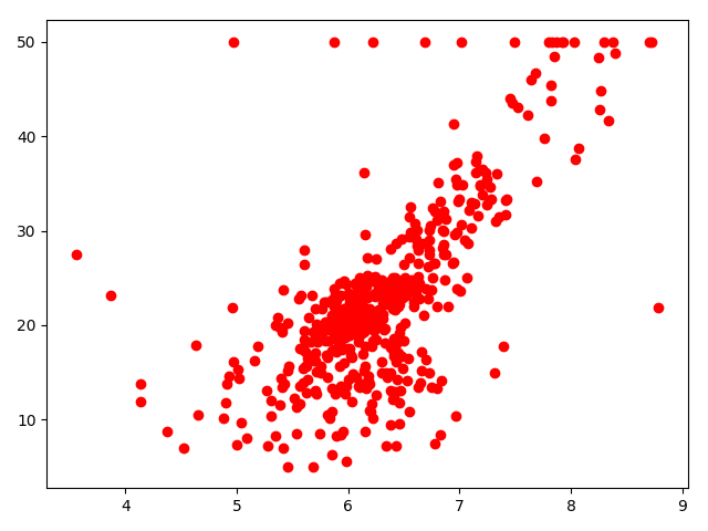
绘制人口中低收入阶层比例与房价关系的散点图:
1
2plt.scatter(x['LSTAT'], y, color='blue')
plt.show()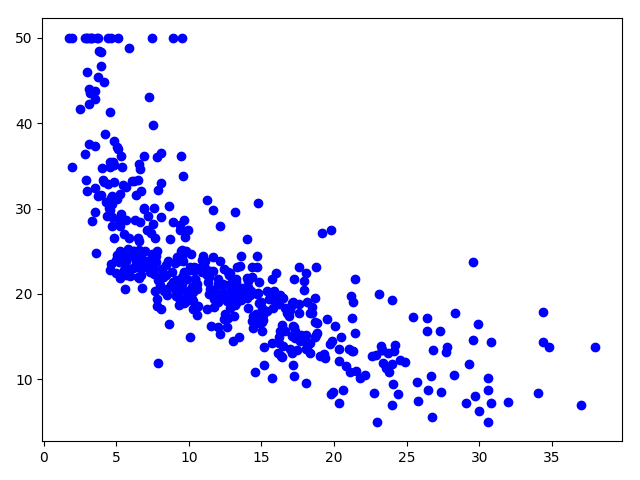
发现基本上存在一定的线性关系,采用线性回归模型尝试。
建模
利用statsmodel.api中的普通最小二乘回归模型拟合
1
2
3
4
5
import statsmodels.api as sm
x_add1 = sm.add_constant(x)
model = sm.OLS(y, x_add1).fit()
print(model.summary())拟合结果:
1
2
3
4
5
6
7
8
9
10
11
12
13
14
15
16
17
18
19
20
21
22
23
24
25
26
27
28
29
30
31
32
33
34
35
36
37
38
OLS Regression Results
==============================================================================
Dep. Variable: MEDV R-squared: 0.741
Model: OLS Adj. R-squared: 0.734
Method: Least Squares F-statistic: 108.1
Date: Sun, 05 May 2019 Prob (F-statistic): 6.72e-135
Time: 22:59:08 Log-Likelihood: -1498.8
No. Observations: 506 AIC: 3026.
Df Residuals: 492 BIC: 3085.
Df Model: 13
Covariance Type: nonrobust
==============================================================================
coef std err t P>|t| [0.025 0.975]
------------------------------------------------------------------------------
const 36.4595 5.103 7.144 0.000 26.432 46.487
CRIM -0.1080 0.033 -3.287 0.001 -0.173 -0.043
ZN 0.0464 0.014 3.382 0.001 0.019 0.073
INDUS 0.0206 0.061 0.334 0.738 -0.100 0.141
CHAS 2.6867 0.862 3.118 0.002 0.994 4.380
NOX -17.7666 3.820 -4.651 0.000 -25.272 -10.262
RM 3.8099 0.418 9.116 0.000 2.989 4.631
AGE 0.0007 0.013 0.052 0.958 -0.025 0.027
DIS -1.4756 0.199 -7.398 0.000 -1.867 -1.084
RAD 0.3060 0.066 4.613 0.000 0.176 0.436
TAX -0.0123 0.004 -3.280 0.001 -0.020 -0.005
PTRATIO -0.9527 0.131 -7.283 0.000 -1.210 -0.696
B 0.0093 0.003 3.467 0.001 0.004 0.015
LSTAT -0.5248 0.051 -10.347 0.000 -0.624 -0.425
==============================================================================
Omnibus: 178.041 Durbin-Watson: 1.078
Prob(Omnibus): 0.000 Jarque-Bera (JB): 783.126
Skew: 1.521 Prob(JB): 8.84e-171
Kurtosis: 8.281 Cond. No. 1.51e+04
==============================================================================
Warnings:
[1] Standard Errors assume that the covariance matrix of the errors is correctly specified.
[2] The condition number is large, 1.51e+04. This might indicate that there are
strong multicollinearity or other numerical problems.训练数据优化
根据上面拟合结果报告,
P>|t|这列中,大于0.005的即为异常值,可以视为不相关,可以剔除该属性。1
x.drop(['AGE', 'INDUS'], axis=1, inplace=True)
重新拟合
1
2
3
x_add1 = sm.add_constant(x)
model = sm.OLS(y, x_add1).fit()
print(model.summary())拟合结果
1
2
3
4
5
6
7
8
9
10
11
12
13
14
15
16
17
18
19
20
21
22
23
24
25
26
27
28
29
30
31
32
33
34
35
36
OLS Regression Results
==============================================================================
Dep. Variable: MEDV R-squared: 0.741
Model: OLS Adj. R-squared: 0.735
Method: Least Squares F-statistic: 128.2
Date: Sun, 05 May 2019 Prob (F-statistic): 5.54e-137
Time: 23:07:23 Log-Likelihood: -1498.9
No. Observations: 506 AIC: 3022.
Df Residuals: 494 BIC: 3072.
Df Model: 11
Covariance Type: nonrobust
==============================================================================
coef std err t P>|t| [0.025 0.975]
------------------------------------------------------------------------------
const 36.3411 5.067 7.171 0.000 26.385 46.298
CRIM -0.1084 0.033 -3.307 0.001 -0.173 -0.044
ZN 0.0458 0.014 3.390 0.001 0.019 0.072
CHAS 2.7187 0.854 3.183 0.002 1.040 4.397
NOX -17.3760 3.535 -4.915 0.000 -24.322 -10.430
RM 3.8016 0.406 9.356 0.000 3.003 4.600
DIS -1.4927 0.186 -8.037 0.000 -1.858 -1.128
RAD 0.2996 0.063 4.726 0.000 0.175 0.424
TAX -0.0118 0.003 -3.493 0.001 -0.018 -0.005
PTRATIO -0.9465 0.129 -7.334 0.000 -1.200 -0.693
B 0.0093 0.003 3.475 0.001 0.004 0.015
LSTAT -0.5226 0.047 -11.019 0.000 -0.616 -0.429
==============================================================================
Omnibus: 178.430 Durbin-Watson: 1.078
Prob(Omnibus): 0.000 Jarque-Bera (JB): 787.785
Skew: 1.523 Prob(JB): 8.60e-172
Kurtosis: 8.300 Cond. No. 1.47e+04
==============================================================================
Warnings:
[1] Standard Errors assume that the covariance matrix of the errors is correctly specified.
[2] The condition number is large, 1.47e+04. This might indicate that there are
strong multicollinearity or other numerical problems.
预测
输出建模结果
coef 列即为计算出的回归系数
1
2
3
4
5
6
7
8
9
10
11
12
13
14
print(model.params)
const 36.341145
CRIM -0.108413
ZN 0.045845
CHAS 2.718716
NOX -17.376023
RM 3.801579
DIS -1.492711
RAD 0.299608
TAX -0.011778
PTRATIO -0.946525
B 0.009291
LSTAT -0.522553
dtype: float64获取测试数据:
1
2
import numpy as np
x_test = np.array([[1, 0.006, 18.0, 0.0, 0.52, 6.6, 4.87, 1.0, 290.0, 15.2, 396.2, 5]])预测
1
2
print(model.predict(x_test))
[29.51617469]