该系列为南京大学课程《用Python玩转数据》学习笔记,主要以思维导图的记录
6.1 聚类分析
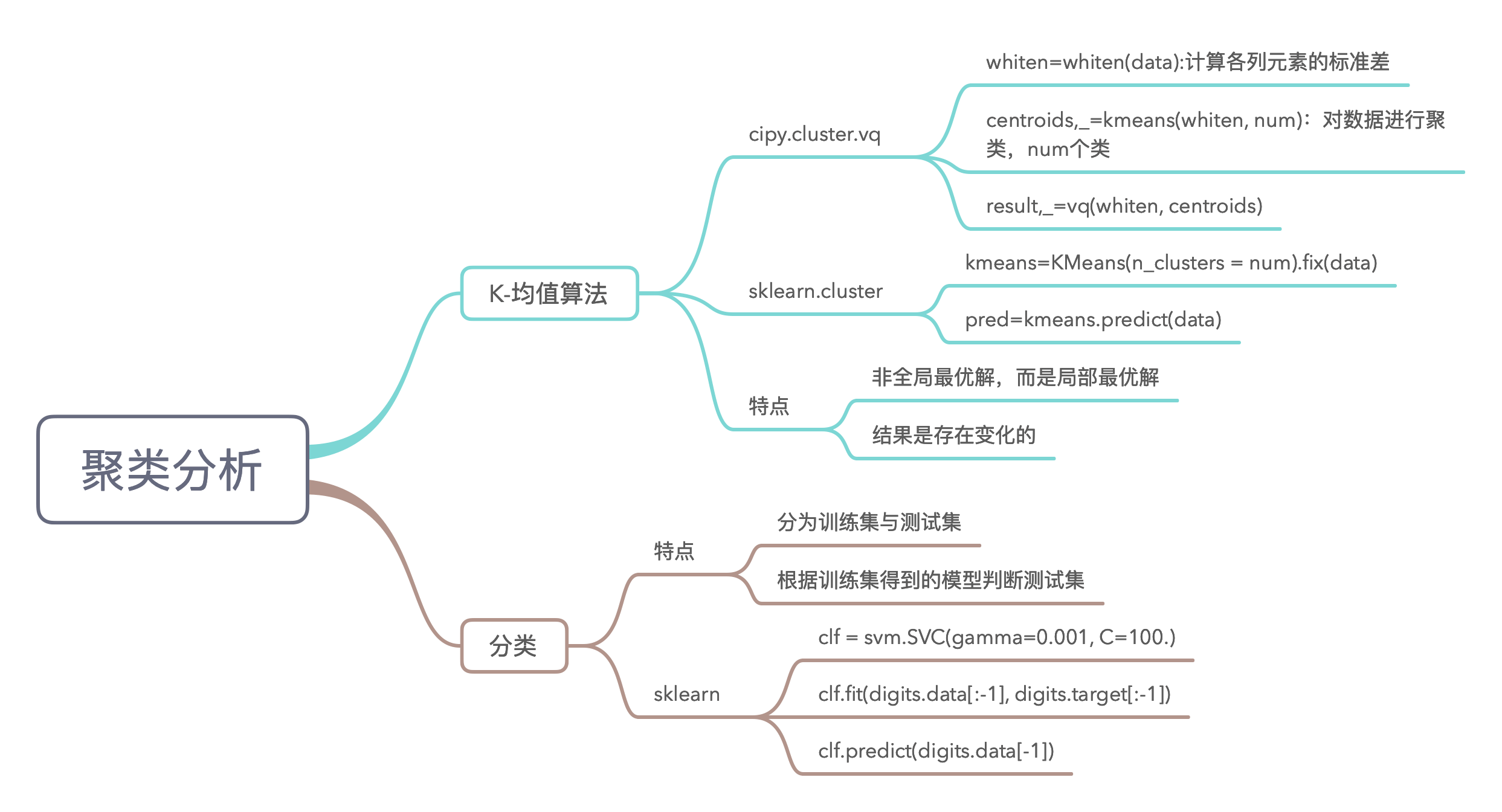
6.1 扩展 scikit-learn 机器学习经典入门项目
scikit-learn 是基于 NumPy、SciPy 和 Matplotlib 的著名的 Python 机器学习包,里面包含了大量经典机器学习的数据集和算法实现,请基于经典的鸢尾花数据集 iris 实现简单的分类和聚类功能。
实现:
1 | # -*- coding: utf-8 -*- |
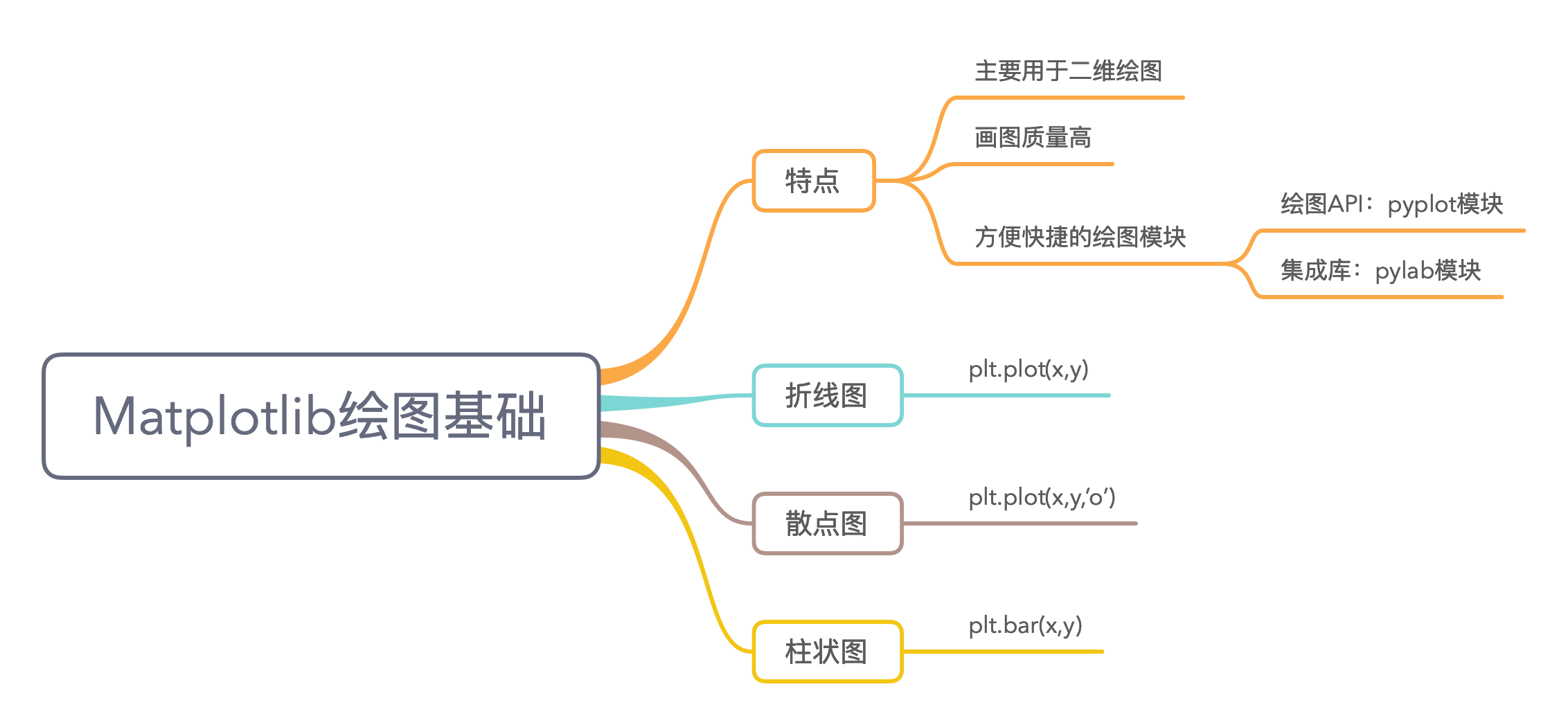
6.2 Matplotlib绘图基础
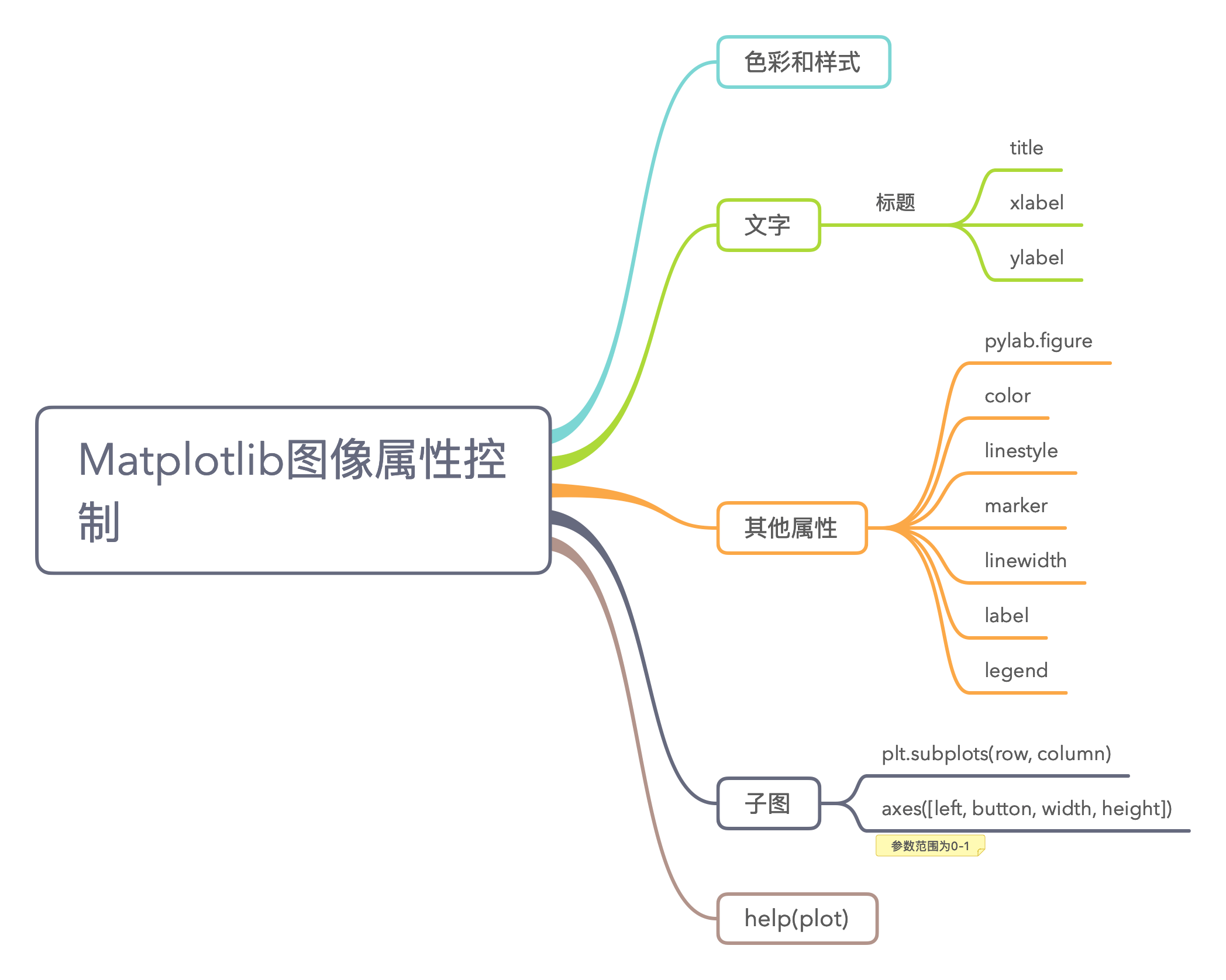
6.3 Matplotlib图像属性控制
6.3 练习
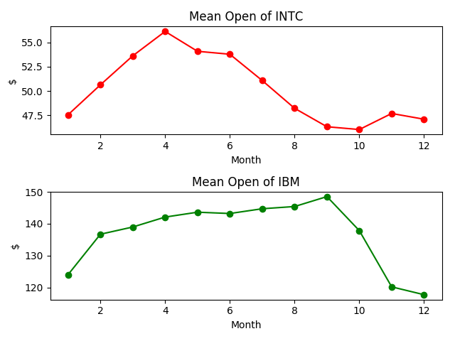
1、数据比较图绘制
请将 Intel 和 IBM 公司近一年来每个月开票价的平均值绘制在一张图中(用 subplot()或subplots()函数)。
实现:
1 | # -*- coding: utf-8 -*- |
结果:
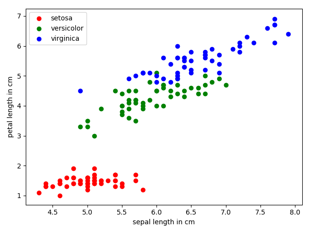
2、iris数据集绘图
利用“6.1 扩展:Scikit-learn 经典机器学习经典入门小项目开发”中介绍的鸢尾花 iris数据集中的某两个特征(例如萼片长度和花瓣长度)绘制散点图。
实现:
1 | # -*- coding: utf-8 -*- |
结果:
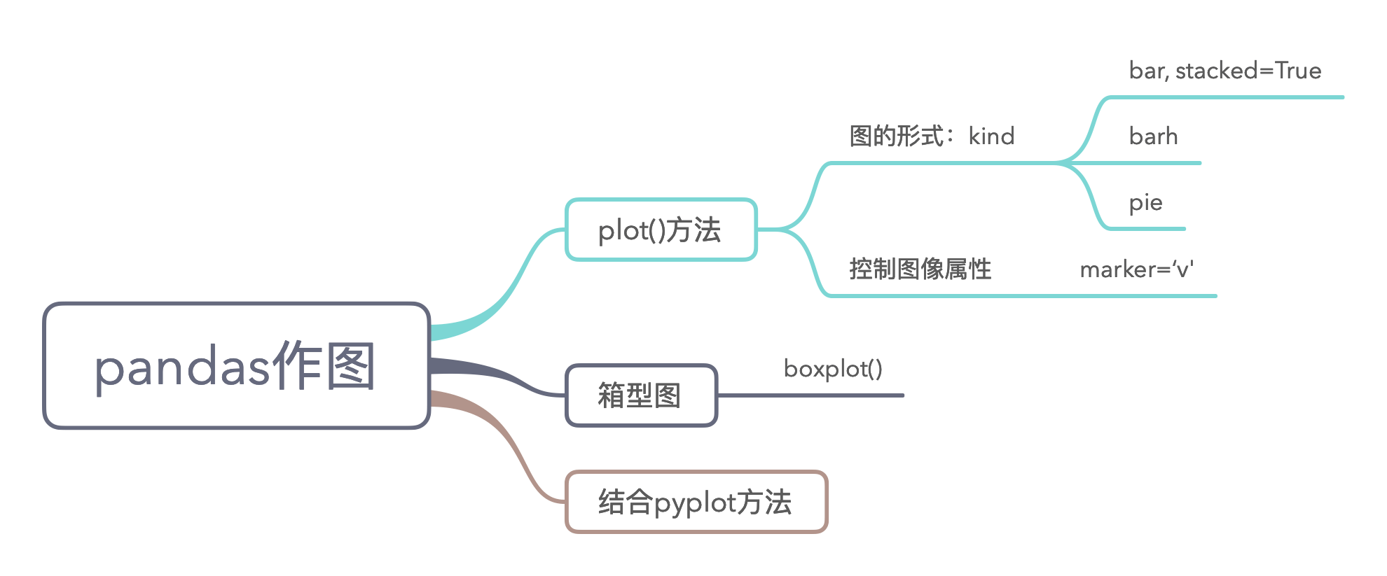
6.4 Pandas作图